
US counties — commuter flows dominate
County-level GTP drill (3,258 counties; commuter-flow tells the story).
An interactive county choropleth is planned; the drill-down below is live.
3,258 counties, part of FAND’s growing subnational coverage below the national balance sheet. Same balance-sheet identity. At this scale, the cross-border story is commuter flows — income earned in one county, spent in another. The economic reality most Americans actually live.
Why counties matter
A bedroom suburb and its downtown neighbor look almost identical on a GDP map — production is captured where the work happens. But on a wealth map they diverge sharply: Manhattan accumulates produced assets and financial wealth; Bergen County accumulates household wealth (housing, education, retirement claims) that the Manhattan-earned income built.
You cannot see this dynamic at the country scale. You cannot see it at the state scale. You can only see it when the unit of measurement is small enough to be on one side or the other of a commuter flow.
The county-level crosstab, through the national lens
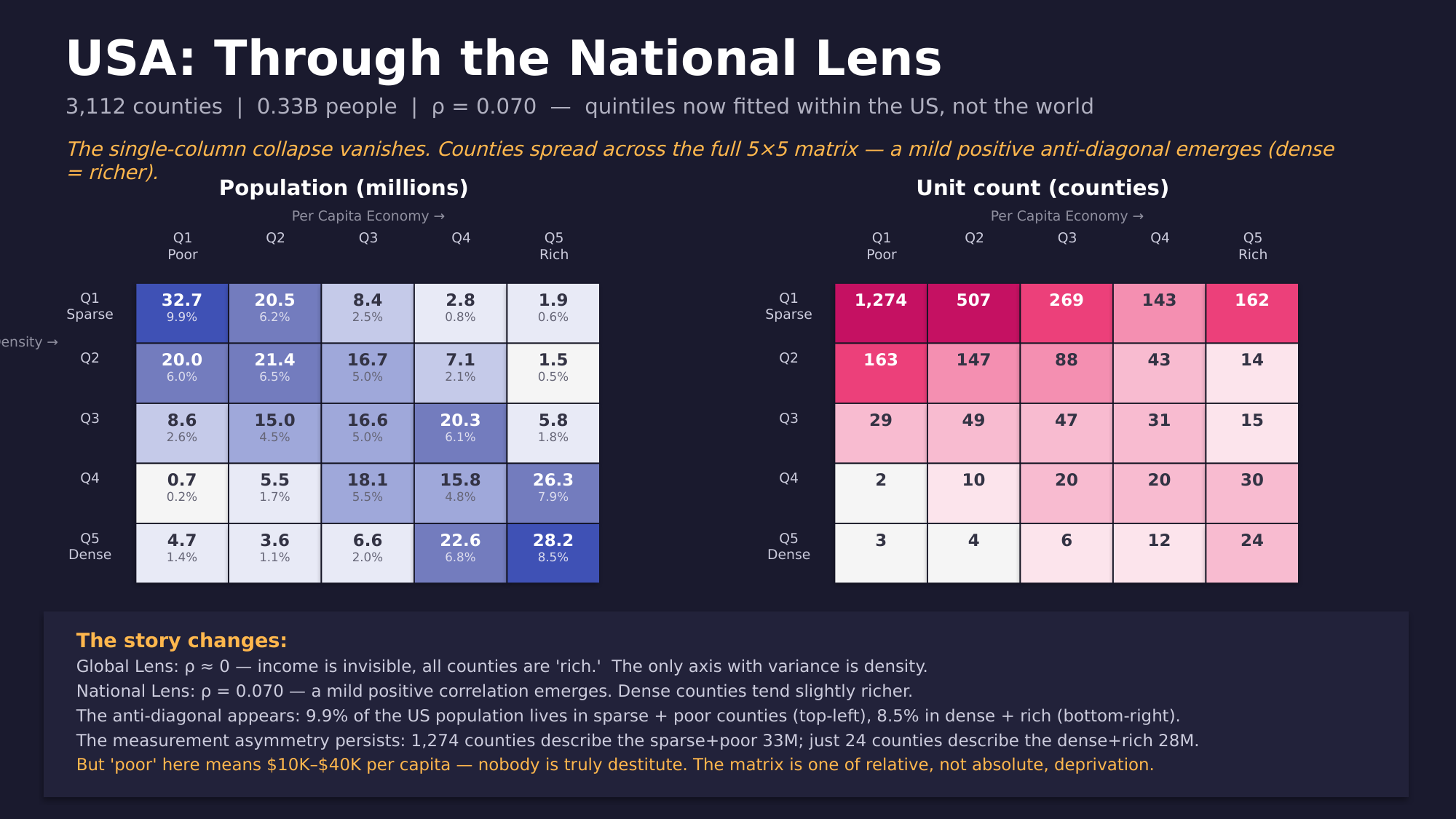
The Global Leaves crosstab places every country’s finest administrative unit on a world-population-weighted grid. Refit that same density × per-capita-income grid to just the 3,112 US counties it can price, and the picture changes:
The deferred-maintenance overlay
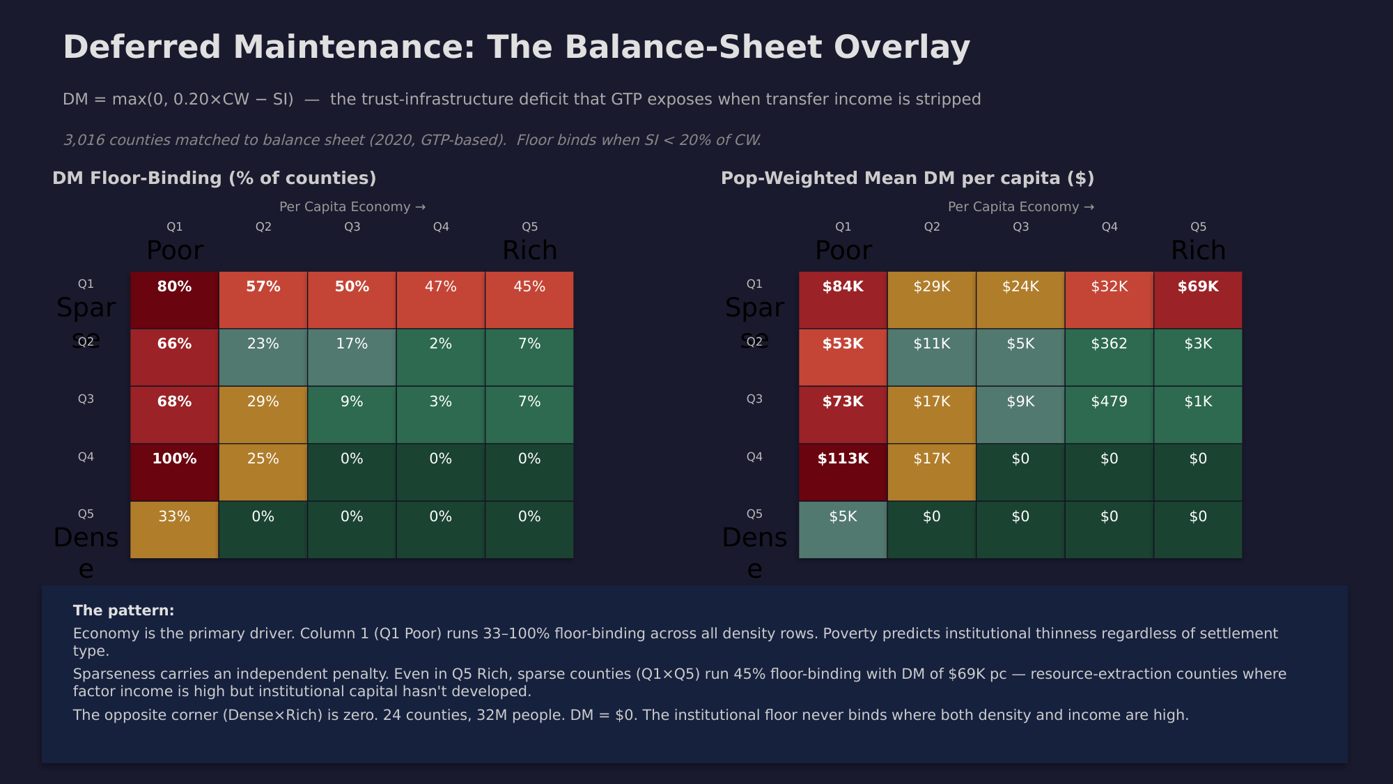
FAND’s Deferred Maintenance (DM) term — the trust-infrastructure deficit exposed when transfer income is stripped from Substantive-Income-based county wealth — floor-binds unevenly across the same grid. It isn’t the same story as density × wealth; it’s the institutional-thinness story layered on top of it.
Related reading
- Global Leaves crosstab — the world-scale version of this same density × wealth grid, and the 38× measurement asymmetry it surfaces globally.
- Five spatial scales — where TL3 (county) sits relative to TL1/TL2, and why cross-border means commuter flows here and interstate flows one level up.
- US states — the same identity one level up, and the gap between the county-built and top-down national record.
What’s here at launch
- County list with balance-sheet drill-down per county (3,258 entries)
- The “GTP” (Gross Territorial Product, HQ-bias corrected) is the income base, not GDP — corrects the systematic distortion that GDP introduces at sub-national scales
- The commuter-flow story foregrounded as the defining relationship at county scale